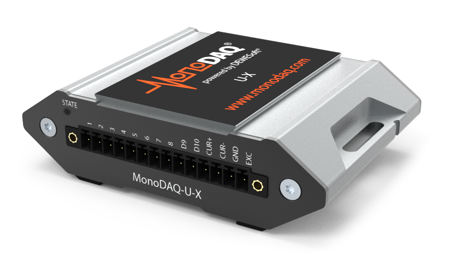
Getting Started with MonoDAQ-U-X
Setting up IDM
Download and install Installation
To start IDM in MAC or Windows just click on the downloaded file. In Linux type java -jar idm.jar. for further instructions please see: IDM Command Line Parameters
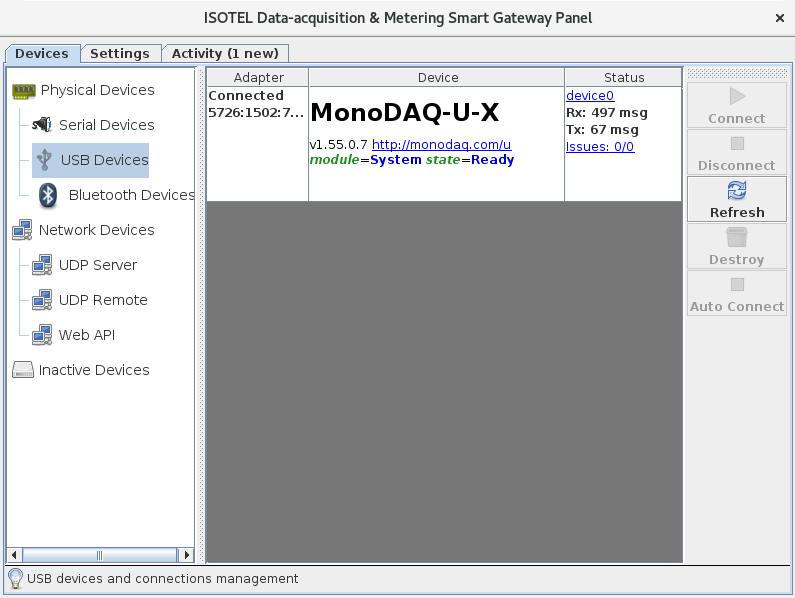
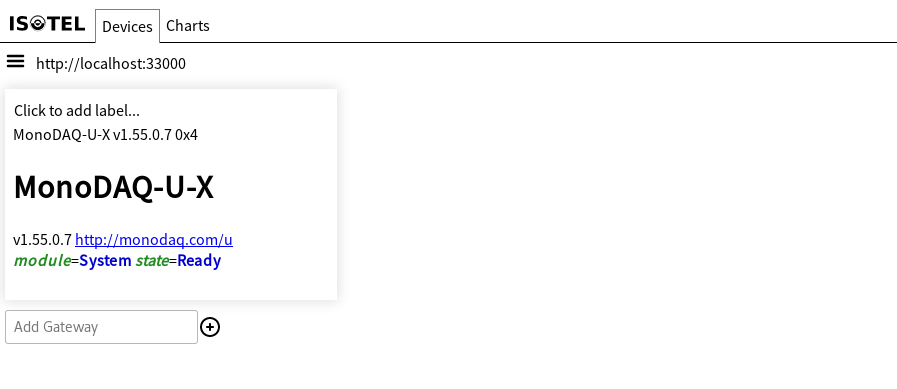
Plug in your MonoDAQ, click on Devices and go to USB devices; you should see it displaying its version and up-to-date status.
Navigating inside IDM
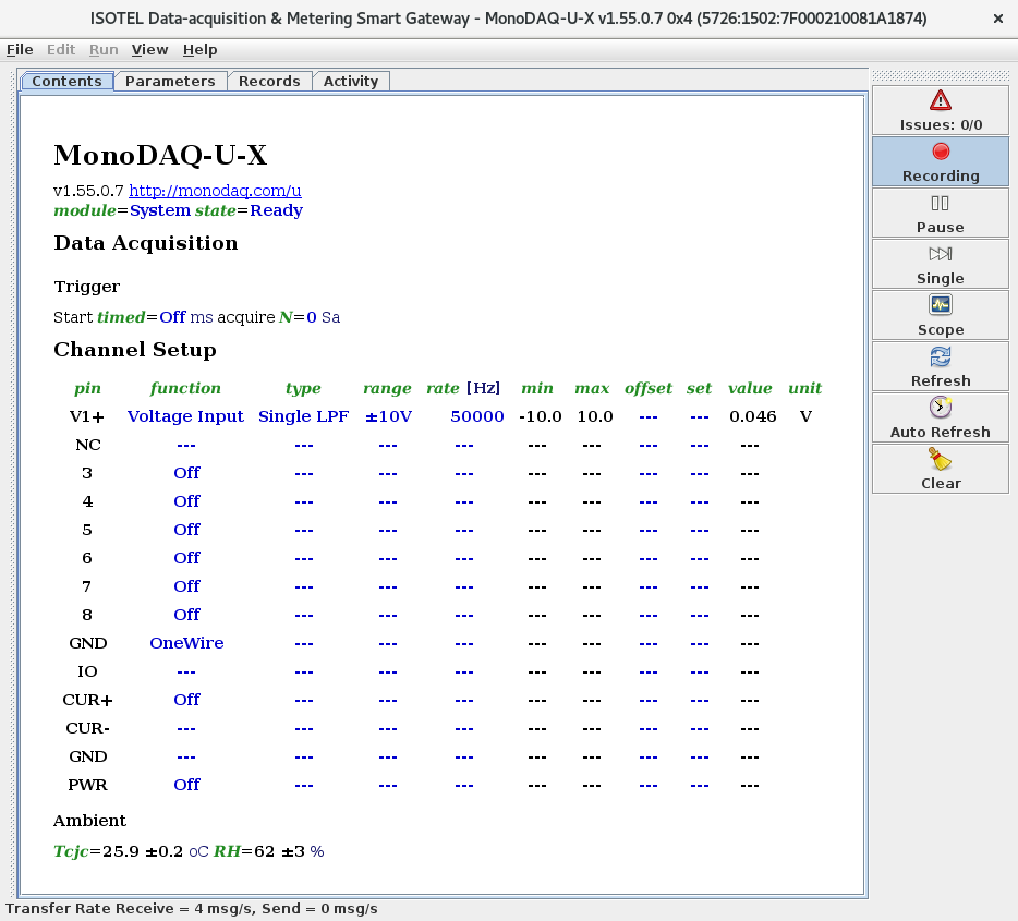
Double clicking on the MonoDAQ-U-X device opens the so-called Device View window in Basic View. For MonoDAQ-U-X this page is also called Channel Setup view. By default, MonoDAQ-U-X presets one voltage channel at the maximum rate. The user can start reconfiguring the channels by simply clicking inside that content. Everything in blue is clickable.
MonoDAQ-U-X will automatically adjust the rate settings or voltage ranges if the desired configuration conflicts with the other settings. During re-configuration you may also check the very top line informing that module = System is state = Ready, which reports the current progress. The measurements are shown in the value column and are updated in real-time.
Parameters Tab
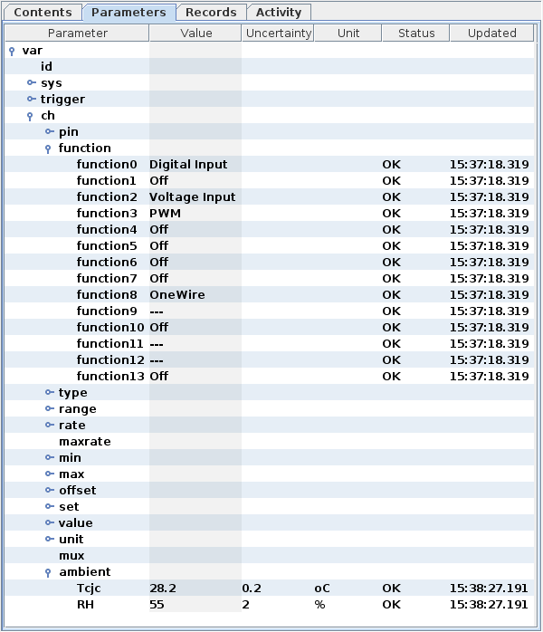
The parameter Tab shows all of the device parameters structured in a tree, with additional information, such as precision, uncertainty where given, unit and time stamp of the last update received.
When accessing parameters via python api, you may use this view to note down the path, i.e., to assign a different function to pin 1, and to read its value:
>>> mdu['ch.function.function0'] = 'Digital Input'
>>> mdu['ch.value.value0']
'0'
Status Reporting
IDM stores everything it receives from MonoDAQ-U-X by default, except the streaming samples. The history of these records can be browsed under the Records Tab.
If an error occurs, the MonoDAQ-U-X title turns red and the Issues button displays the number of errors. Clicking on it will highlight the parameters that reported a problem. For a deep diagnosis, the user may need to change the Basic View into a more detailed view, which can be done in the View menu.
Embedded Operation and Remote Control
IDM can run as a deamon on Raspberry PI, NAS or other systems supporting java. The status reporting integrates with a standard syslog and IDM also starts Web API by default. By visiting the web view app at http://idm.isotel.eu you can easily access MonoDAQ-U-X, monitor and control it remotely.
All the information from the Channel Setup is recorded, meaning that the web view app offers a simple way to plot temperatures from thermocouples, or other channels, by simply clicking on a parameter and adding it to the chart.
Real Power comes with Python and Jupyter
Assuming you are familiar with python and have already installed it, install isotel-idm package with:
pip install jupyter bokeh isotel-idm
to get full MonoDAQ-U-X support. Learn more under Python & Jupyter Support.
The isotel-idm package is best described in the following
Jupyter Getting Started Notebook:
Getting Started with MonoDAQ
We will walk you through the basic usage of python API, like how to:
- setup channels,
- fetch values,
- plot it,
- add a math channel and
- run it as a real-time scope with a rising edge trigger.
Wiring
In this demo we shall activate an analog, a digital one and a PWM channel, then wire the PWM output (from pin 4) back to the digital input (pin 1).
1. Setup Channels
First we call the reset() function to begin from the start, then we configure the channels, and print out the configuration. The configuration could also be stored in a 1-wire memory attached to a connector that is automatically reloaded when the connector with such a memory is detected.
When directly accessing the parameters, you may want to use the Parameters view of the IDM, which will help you browse through the device data structure.
from isotel.idm import monodaq, signal, gateway

mdu = monodaq.MonoDAQ_U()
mdu.reset()

mdu['ch.function.function3'] = 'PWM'
mdu['ch.rate.rate3'] = 1200
mdu['ch.set.set3'] = 0.25

mdu['ch.function.function0'] = 'Digital Input'
mdu['ch.function.function2'] = 'Voltage Input'
mdu['ch.rate.rate2'] = 50000

mdu.wait4ready()
mdu.print_setup()
2. Acquire Only
The MonoDAQ_U.fetch() method is a python generator and fetches N samples from analog channels or digital ones if the analog channels are not active to return the stream of tuples organized as:
- tuples of independent streams,
- each stream holds time (x-axis) and the tuple of channels synchronous to the time (y-axis),
For example:
s[0][1][0]means from stream0, channels, and select 0-th channel
The generator provides meta information on the channels in the first line (row). In order to fetch the values, the generators need a sink, which loops over all the entries. In our example, we simply use the list() as the sink to display values.
From the channel setup above, we can see that digital samples run twice as fast as analog ones. However since N primarily selects analog samples, the following example will put twice the number of digital samples compared to analog ones:
list( mdu.fetch(N=3) )
3. Plot
The fetch() method outputs a stream. To be able to plot it, the stream must be collected into a signal. A signal here means a dict sorted by channels, each having a pair of lists of equal size, providing Y samples and corresponding X time samples.
To convert the generated output to a stream use the signal.stream2signal() method, which is a generator returning signals.
By extending this example we get a nicely sorted dict; again we use the list() to display the results. We may again observe more digital samples than analog ones, however, the time axis fits together nicely:
list( signal.stream2signal( mdu.fetch(3) ))
Now to the plot, with the signal.scope() which iterates over signals provided by the stream2signal() method and returns last acquired signal as data. Let us increase the number of samples to get a nicer waveform.
signal.scope( signal.stream2signal( mdu.fetch(100) ), title = 'First Plot');
4. Adding a Math Channel
It would be a pity not to be able to perform a real-time analysis or computation on data in python.
We mute the first V1+ [V] channel and change the colors of the other two. You may freely enter
an equation with channel names with big capital letters, and only up to the + sign or space.
signal.scope(
    signal.stream2signal(
        signal.addmath( mdu.fetch(100), 'Masked [V]', expr = '5*V1*DI1'),
    ), title = 'First Plot with Math Channel', colors = [ None, 'darkgreen', 'darkorange']);
5. Real-time Scope
Real-time updates require that a larger continuous stream of samples is fetched from the MonoDAQ. We achieve that by providing fetch(2000000) a sufficiently big number to run for some more time.
To display the intermediate collected samples, we need to instruct the stream2signal() a split parameter with a number of samples to be displayed in one shot. Note that fetch() refers to analog samples and there may be a significantly larger number of digital samples at the output. In addition if you want, you can reset the time and start at zero each time a shot is made. Then you should set the relative_time to True.
And last, we introduce a rising edge trigger function signal.trigger, which evaluates:
- The precondition that must be met in order to search for a
- trigger condition.
- Trigger is set a
single_shotmode by default.
The example below shows how to wait for a rising edge on the DI1 digital channel by specifying both the pre-condition and the condition. When the condition triggers, P pre-buffered samples are yielded and then continues for the remaining N samples.
data = signal.scope(
    signal.stream2signal(
        signal.trigger( mdu.fetch(2000000), precond='DI1 < 0.5', cond='DI1 > 0.5',
                        P=200, N=200, single_shot=False, post_delay = 0.1),
        split=400, relative_time=True),
    title="Continous Mode - Rising Edge Trigger", y_range = (-0.1,1.1) )
if not data:
    print('Signal not detected')
MonoDAQ-U-X Command Line Interface
On embedded systems, like Raspberry PI, or even desktop, you may want to have a CLI control over the device. The monodaq module within the isotel-idm provides:
$ python -m isotel.idm.monodaq -h
usage: monodaq.py [-h] [--gateway GATEWAY] [-d D] [-N N] [-s S [S ...]]

MonoDAQ-U-X Utility 1.0a11

optional arguments:
-h, --help         show this help message and exit
--gateway GATEWAY  gateway address, defaults to http://localhost:33000
-d D               Device to fetch from, like: 'MonoDAQ-U-X v1.55.0.17 0x4'
                    or just: device0
-N N               Fetch N samples and print results in TSV format
-s S [S ...]       Set or query a parameter, like: ch.function.function0
                    'Digital Input'
To list all available devices type (or optionally provide a –gateway):
$ python -m isotel.idm.monodaq
device0      MonoDAQ-U-X v1.55.0.17 0x4
To see the Channel Setup:
$ python -m isotel.idm.monodaq -d device0
|pin           |function      |type          |range         |rate [Hz]     |min           |max           |offset        |set           |value         |unit          |
|--------------|--------------|--------------|--------------|--------------|--------------|--------------|--------------|--------------|--------------|--------------|
|DI1           |Digital Input |TTL           |5 V           |100000        |0             |5             |---           |---           |5             |V             |
|2             |Off           |---           |---           |---           |---           |---           |---           |---           |---           |              |
|V1+           |Voltage Input |Single Ended  |2V            |50000         |-0.1          |2.0           |---           |---           |0.0439        |V             |
|PWM4          |PWM           |TTL           |5 V           |1200          |0.00          |0.83          |---           |0.25          |---           |ms            |
|5             |Off           |---           |---           |---           |---           |---           |---           |---           |---           |              |
|6             |Off           |---           |---           |---           |---           |---           |---           |---           |---           |              |
|7             |Off           |---           |---           |---           |---           |---           |---           |---           |---           |              |
|8             |Off           |---           |---           |---           |---           |---           |---           |---           |---           |              |
|GND           |OneWire       |---           |---           |---           |---           |---           |---           |---           |---           |              |
|IO            |---           |---           |---           |---           |---           |---           |---           |---           |---           |              |
|CUR+          |Off           |---           |---           |---           |---           |---           |---           |---           |---           |              |
|CUR-          |---           |---           |---           |---           |---           |---           |---           |---           |---           |              |
|GND           |---           |---           |---           |---           |---           |---           |---           |---           |---           |              |
|PWR           |Off           |---           |---           |---           |---           |---           |---           |---           |---           |              |
To fetch 10 samples and print them on screen. Note that the t character may not perfectly align the spacing between the numbers, however the single t simplifies parsing and importing into LibreCalc or Excel. To redirect them to a file add > file.tsv at the end.
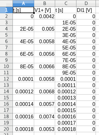
$ python -m isotel.idm.monodaq -d device0 -N 10
t [s]       V1+ [V] t [s]   DI1 [V]
0.0 0.1738  0.0     1
        1e-05       1
2e-05       0.1599  2e-05   1
        3e-05       1
4e-05       0.1559  4e-05   1
        5e-05       1
6e-05       0.1422  6e-05   1
        7e-05       1
8e-05       0.1386  8e-05   1
        9e-05       1
0.0001      0.1226  0.0001  1
        0.00011     1
0.00012     0.1241  0.00012 1
        0.00013     1
0.00014     0.0721  0.00014 1
        0.00015     0
0.00016     -0.0529 0.00016 0
        0.00017     0
0.00018     -0.0379 0.00018 0
To change input on the 1st channel by its unique name rather than device0:
$ python -m isotel.idm.monodaq -d 'MonoDAQ-U-X v1.55.0.17 0x4' -s ch.function.function0 'Voltage Input'
Voltage Input
or to obtain reading, i.e. of humidity, or a value from the 1st voltage channel:
$ python -m isotel.idm.monodaq -d 'MonoDAQ-U-X v1.55.0.17 0x4' -s ch.ambient.RH
56.0+/-2.0

$ python -m isotel.idm.monodaq -d 'MonoDAQ-U-X v1.55.0.17 0x4' -s ch.value.value0
2.4533
However you can combine the IDM Web View (http://idm.isotel.eu) to configure and review the Channel Setup with the CLI to fetch samples into TSV formatted file. Note that if your IDM is configured in non-TLS mode, then the the isotel.net must be also open in non-TLS the http://… mode and not the https://… in order to be able to access MonoDAQ-U devices.
Fetching Recorded Samples
IDM by default stores all the monitoring data to record files, except the streaming data. To fetch recorded samples from say channel 0 from a remote server, say NAS or RPi:
$ python -m isotel.idm.monodaq --gateway http://192.168.0.106:33000 [--user admin] [--pass X] -d device0 -s ch.value.value0 --to last -N 5
1560002647.066    0.005
1560002648.066    0.006
1560002649.066    0.005
1560002650.066    0.006
1560002652.066    0.006
Optionally username and password must be given if enabled in the IDM.
To fetch all channels at once, root structure is given instead of the individual channel:
$ python -m isotel.idm.monodaq --gateway http://192.168.0.106:33000 -d device0 -s ch.value --to last -N 5
1560002256.094    0.006    ---    ---    0    -1424.6    ---    0    ---    ---    ---    0.0    ---    -0.03    10.999
1560002257.094    0.006    ---    ---    0    -1424.6    ---    0    ---    ---    ---    0.0    ---    -0.03    10.999
1560002257.095    0.006    ---    ---    0    -1424.6    ---    0    ---    ---    ---    0.0    ---    -0.03    11.000
1560002258.094    0.005    ---    ---    0    -1424.6    ---    0    ---    ---    ---    0.0    ---    -0.03    11.000
1560002259.094    0.005    ---    ---    0    -1424.6    ---    0    ---    ---    ---    0.0    ---    -0.03    11.000
The interval of interest is set with the –to and –from parameters. Saying –to last will position at the end of records and retrieve -N samples from the back. One may use the –scale N parameter to reduce (down-sample) the number of samples in given interval down to N. Aliasing may occur. The –to and –from accept time in UTC format as given at the output.